PaperOps: run experiments and add results to a PDF with a single Make command

In my work as research faculty and a PhD supervisor, I constantly try to streamline the research process. Much of that work involves automating running (or re-running) of experiments so that we can quickly test new hypotheses, change parameters, or even just change colors in a figure.

My most recent project has been to develop a simple proof-of-concept in which every aspect of running results to including them in a paper is automated. Simply download the repo from GitHub, run make paper, and it outputs a PDF file with the results from some simple experiments.

The Demo

After pulling the repository and moving to that directory, we can run:

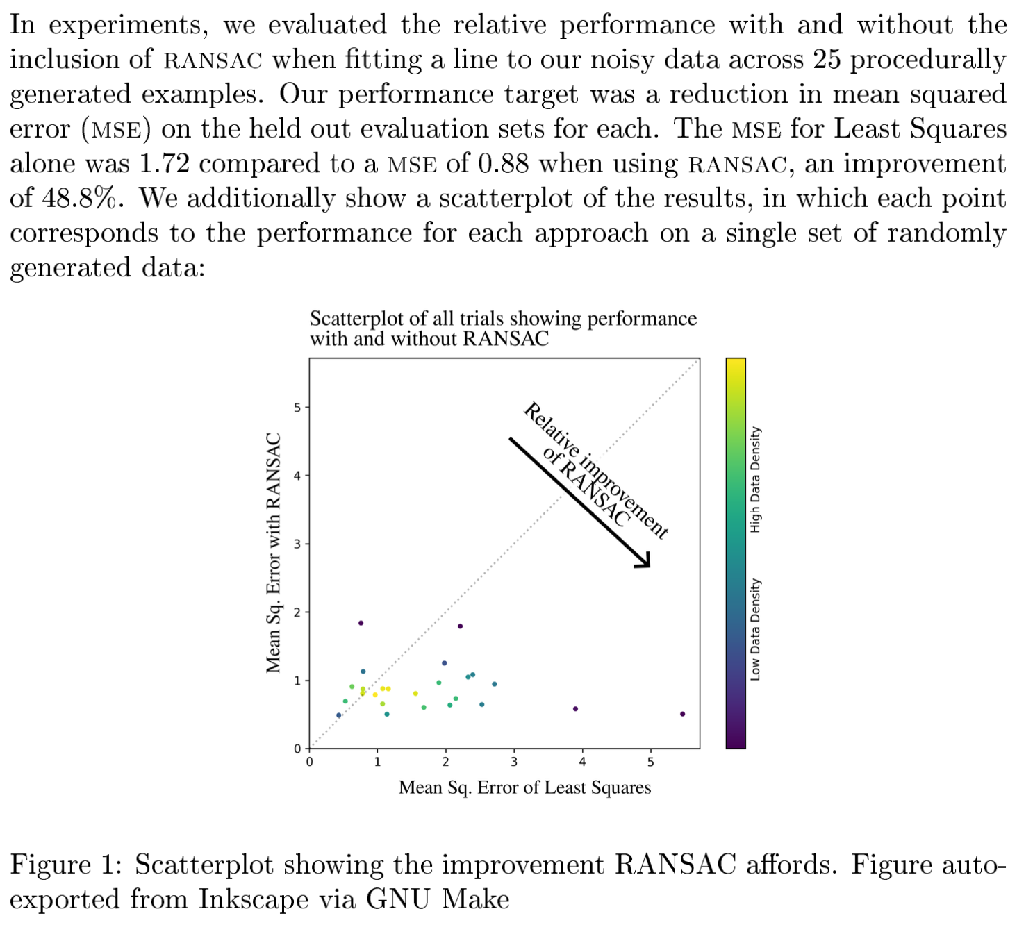
make paper NUM_EXPERIMENTS=25

This simple command runs 25 “experiments”—a simple example task that fits a line to noisy data with and without outlier rejection and compares the two—and generates a plot that contains a scatter plot of those results and computes statistics for the results. This results in the following PDF, manually cropped to highlight the important bits:

Make paper: 25 experiments. The PDF includes the correct number of experiments, statistics, and a scaterplot of those results, all via make paper NUM_EXPERIMENTS=25. Make paper: 25 experiments. The PDF includes the correct number of experiments, statistics, and a scaterplot of those results, all via make paper NUM_EXPERIMENTS=25.

The PDF includes the number of experiments run, the mean performance with and without outlier rejection, and a scatter plot of the results: all of which are automatically read from the results and included when the PDF is generated via LaTeX.

Let’s say we now wanted more experiments. No problem! We run the command again, but increasing that parameter and add a -j20 for convenience so that the experiments run 20-at-a-time in parallel:

make paper NUM_EXPERIMENTS=800 -j20

which results in the following:

Make paper: 800 experiments. The PDF includes the correct number of experiments, statistics, and a scaterplot of those results. Make paper: 800 experiments. The PDF includes the correct number of experiments, statistics, and a scaterplot of those results.

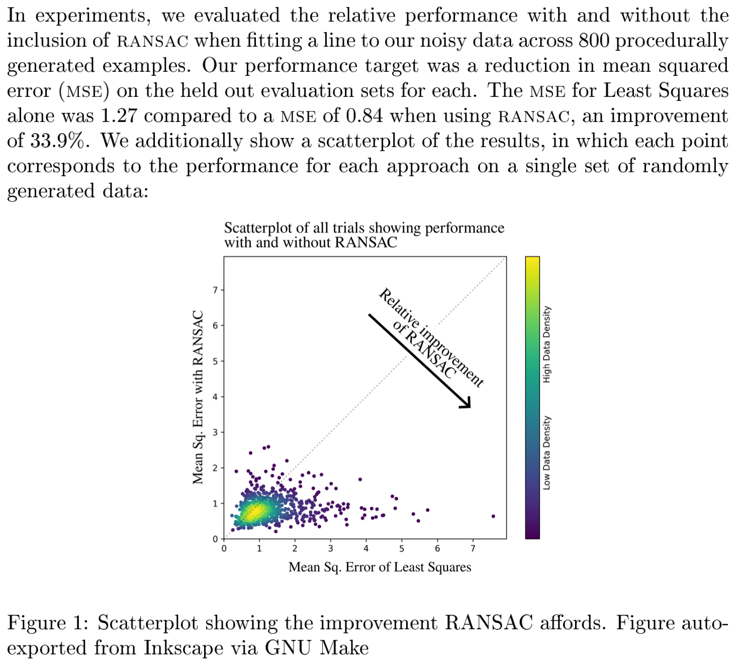
Notice that all the relevant information has been updated automatically, including the plot and the number of experiments and statistics. This is because make takes care of updating the scatterplot as necessary to reflect the updated results and including the newly-computed statistics.

What happens if we rerun the command?

make paper NUM_EXPERIMENTS=800 -j20

We get the following:

make: Nothing to be done for `paper'.

make is designed so that it doesn’t redo computation. Since no new results have been added or changes made, the paper is already up-to-date and nothing needs to be done.

How does it all work? Take a look at the code or read on to learn more.

High-level overview of the process

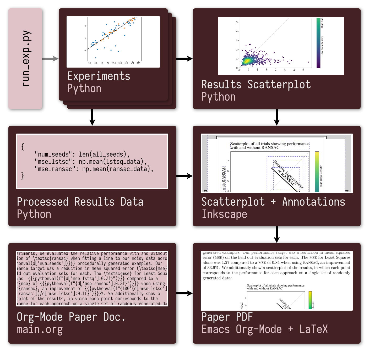
We rely on GNU Make to build the outputs. Upong running make paper all targets upon which the paper relies—including things like the results statistics and the scatterplot—are generated. To generate those, the outputs upon which they rely are also generated, a process that repeats all the way back to the underlying experiments, run automatically to generated the

The following schematic of the dependency structure of the Makefile and so an overview of the outputs generated automatically to build the PDF of the paper:

A schematic of the Make target dependencies. This schematic shows how the different outputs from the code, including the paper itself, depend on others. When running make paper, all upstream outputs are built as necessary to get the results the paper requires. A schematic of the Make target dependencies. This schematic shows how the different outputs from the code, including the paper itself, depend on others. When running make paper, all upstream outputs are built as necessary to get the results the paper requires.

Run experiments with GNU Make

While the fundamentals of GNU Make are beyond the scope of this post, we take advantage of some fairly-specific setup to support changing the number of experiments.

The Make “target” is what is called whenever we want to generate a result. Let’s say we wanted to generate a result for random seed 105 using the least squares line fitting method, accomplished via

make results/results_lstsq_105.csv

We use the % wildcard character to define the Make target and use some simple string processing (via grep) to extract the seed and curve fitting approach from the name of the intended file:

results/results_%.csv: seed = $(shell echo $@ | grep -Eo '[0-9]+' | tail -1)
results/results_%.csv: approach = $(shell echo $@ | grep -Eo '(lstsq|ransac)' | tail -1)
results/results_%.csv:
        @echo "Evaluating result for $(approach): $(seed)\n"
        @mkdir -p results/
        @$(DOCKER_BASE) python3 /src/evaluate_approach.py \
                --seed $(seed) --approach $(approach)

The Python script here is just a simple example, meant to show how extracting some information from the name of the file to be generated can be passed as inputs to the script.

We separately define two variables in Make that automatically populate two lists with all the file names that we would like generated, corresponding to NUM_EXPERIMENTS experiments for each of the least squares (lstsq) and ransac outlier rejection (ransac) line fitting strategies:

eval-lstsq-seeds = \
        $(shell for ii in $$(seq 10000 $$((10000 + $(NUM_EXPERIMENTS) - 1))); \
                do echo "results/results_lstsq_$${ii}.csv"; done)
eval-ransac-seeds = \
        $(shell for ii in $$(seq 10000 $$((10000 + $(NUM_EXPERIMENTS) - 1))); \
                do echo "results/results_ransac_$${ii}.csv"; done)

Now, if we had a separate make target that depended on eval-lstsq-seeds, it would automatically generate all those experiments before it could be run. Adding dependencies like this allows us to enforce that all experiments be finished before we try to perform operations to compute statistics from the data or generate the scatterplot.

Process results and output figures

Generating results and statistics requires a few more Make targets. For example, here is the Make target used to generate the scatterplot via Python:

results/processed_scatterplot.png: src/process_results.py $(eval-lstsq-seeds) $(eval-ransac-seeds)
	@echo "Generating the results scatterplot."
	@$(DOCKER_BASE) python3 /src/process_results.py --output scatterplot

This yields the following figure:

The scatterplot automatically output from Python. Note that it lacks the annotations that appear in the examples above. The scatterplot automatically output from Python. Note that it lacks the annotations that appear in the examples above.

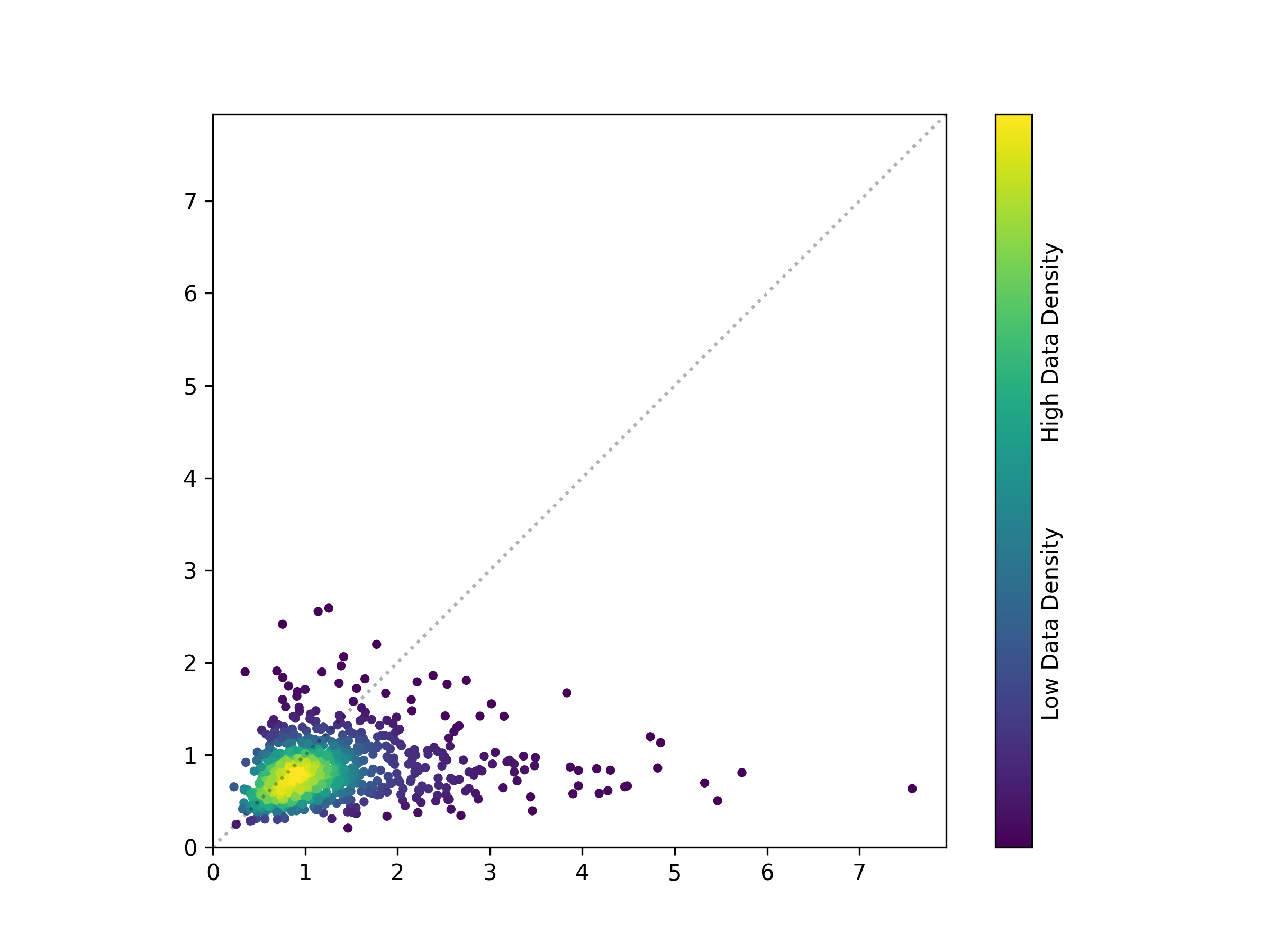
You might notice that the figure lacks the annotations that appear in the PDF. It is often unrealistic to add every annotation and highlight in the Python specification, and so other design software is often used to include such additions by hand, manually placing annotations and text where appropriate to make an effective figure.

For those of you who have used Python’s Matplotlib to make figures, you will understand why trying to place every bit of text or annotation with code is typically non-ideal, often requiring far more time and effort than simply drawing a circle and adding a text box in some other program.

For those of you who have used Python’s Matplotlib to make figures, you will understand why trying to place every bit of text or annotation with code is typically non-ideal, often requiring far more time and effort than simply drawing a circle and adding a text box in some other program.

We use Inkscape—a free and open source vector design software—to add annotations to the figure. Inkscape, like other design software, supports linking resources: the Inkscape .svg file includes only a reference to the underlying scatterplot, so that the Inkscape version of the figure will reflect any changes to the linked images. The Inkscape document uses the underlying scatterplot and includes annotations:

Scatterplot with annotations from Inkscape. Scatterplot with annotations from Inkscape.

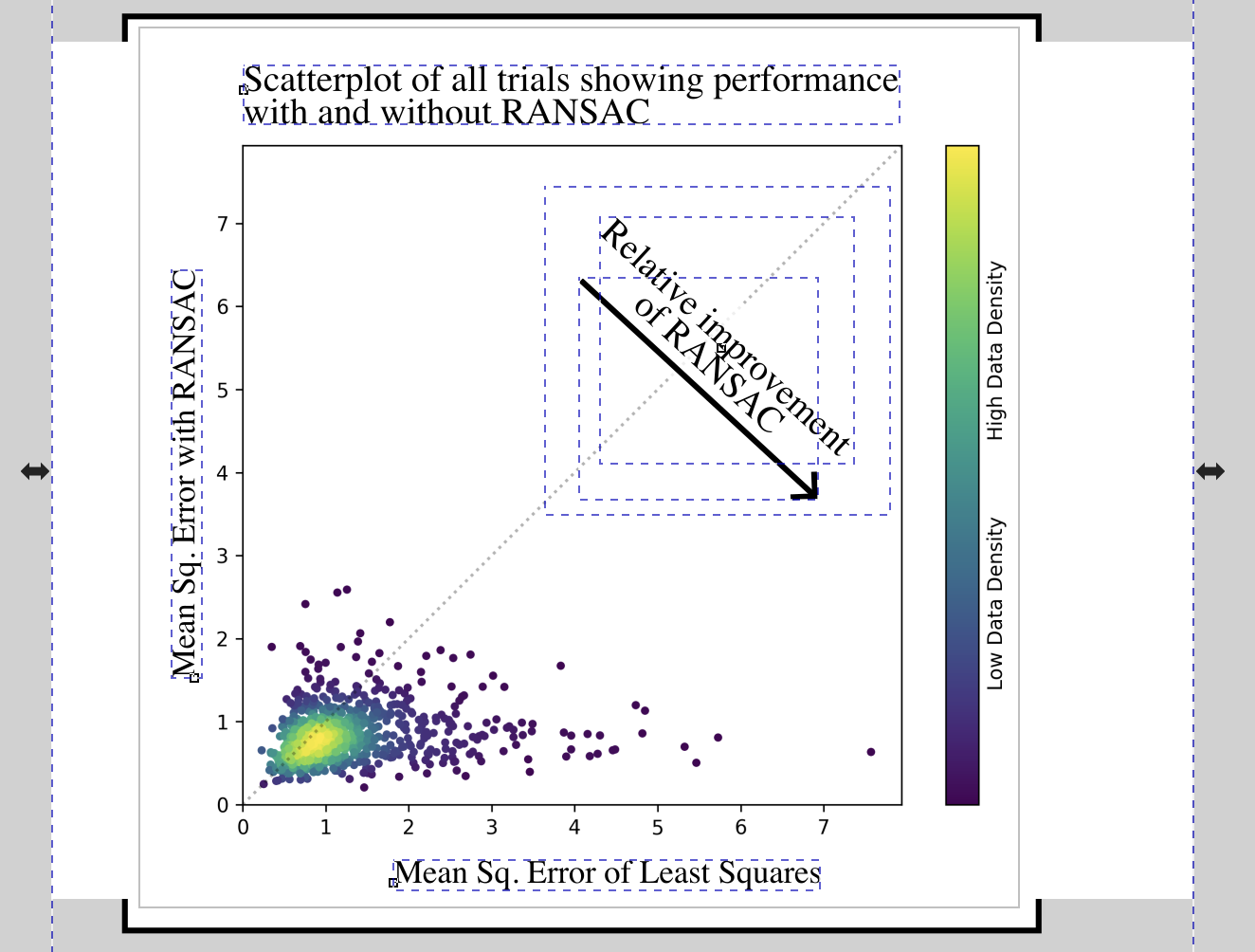
We have a separate Make target that converts the .svg Inkscape file to a .png, so that it may be included in the PDF document later on. For this purpose, we run a headless instance of Inkscape inside a Docker container, avoiding the need to find or run a local instance of Inkscape.

Adding result statistics to the PDF

On Using Pure LaTeX: I show off Emacs here, since it is what I use when composing papers, but there are pure LaTeX solutions to this problem. See this Stack Overflow post about how to use the datatool package for this purpose.

On Using Pure LaTeX: I show off Emacs here, since it is what I use when composing papers, but there are pure LaTeX solutions to this problem. See this Stack Overflow post about how to use the datatool package for this purpose.

In this demo, I use Emacs’ Org-mode as a markup language to compose the paper. Org-mode is a powerful and customizable note taking environment that lets me write a document in a fairly simple syntax and then export it to a .tex file, from which a PDF can be generated. In addition, Org-mode lets me run arbitrary Python code upon export, letting me load a Python .pickle file from data and incorporate the data contained within in the document.

Here is a simple example with code from the paper that: (1) defines the pythonval macro for printing values from Python; (2) defines some LaTeX-specific export options; (3) runs a src block that loads the data file output from our Python commands above; and (4) includes some exmple text:

* LaTeX Configuration :noexport:

#+macro: pythonval src_python[:session :results raw]{$1}
#+LATEX_CLASS_OPTIONS: [10pt]

#+begin_src python :session :results none :exports none
import pickle
with open("../results/processed_results_data.pickle", 'rb') as handle:
    d = pickle.load(handle)
#+end_src

* Some text for the paper

We ran {{{pythonval(d['num_seeds'])}}} experiments 
and saw an improvement of {{{pythonval(f"{100*(d['mse_lstsq'] - 
d['mse_ransac'])/d['mse_lstsq']:0.1f}")}}}%.

Exporting this code to a PDF, the resulting .tex file includes the values computed via python and so yields the examples above.

Conclusion: automation in the RAIL Group

This pipeline gives an overview of how we automate and streamline experimentation in my research lab. We routinely build research pipelines around automated running of experiments as necessary. This level of automated running of experiments dramatically helps facilitate the trying of new ideas. Not only has it proven an effective tool for reproducible research, but also it has made it easy to quickly run additional experiments in the run up to a paper deadline and generate new results in response to reviewers.

See also our lab’s public code repository for examples of our Make- and Docker-based workflow in practice.

Any questions or comments, feel free to reach out to me on Twitter.