Data-Efficient Policy Selection for Navigation in Partial Maps
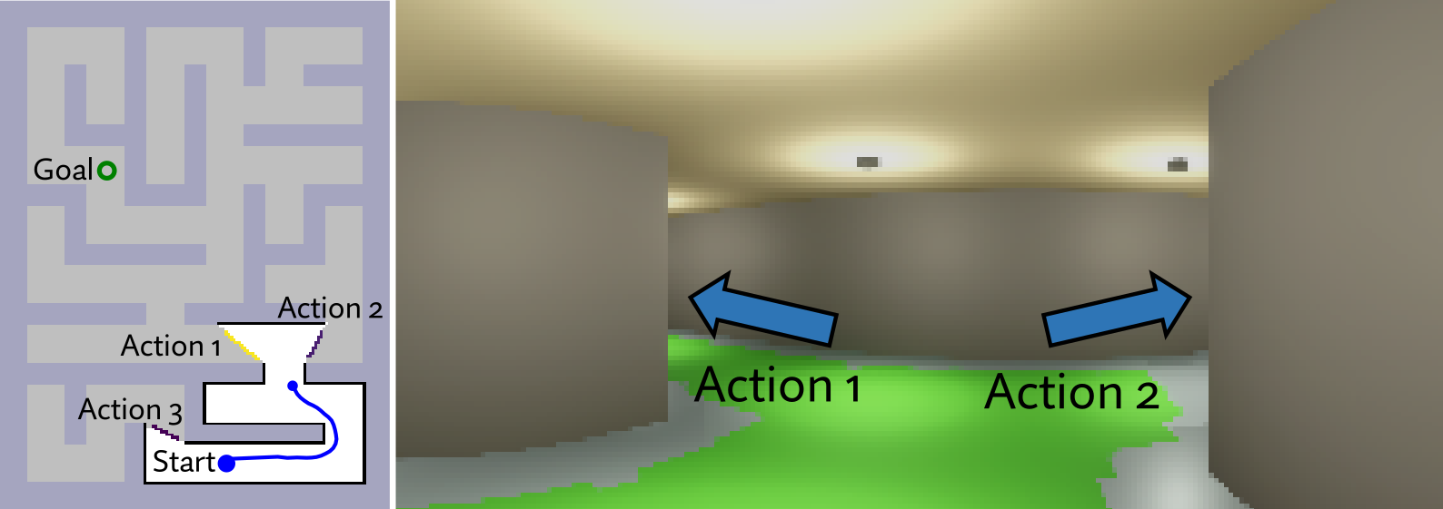
Consider a robot that is tasked to navigate to an unseen goal in a maze in which a green path on the floor signals the route to the goal. The robot’s behavior is guided by a policy that determines what action the robot should take at any point during navigation. In the figure below, the robot comes across a fork while trying to find the goal:
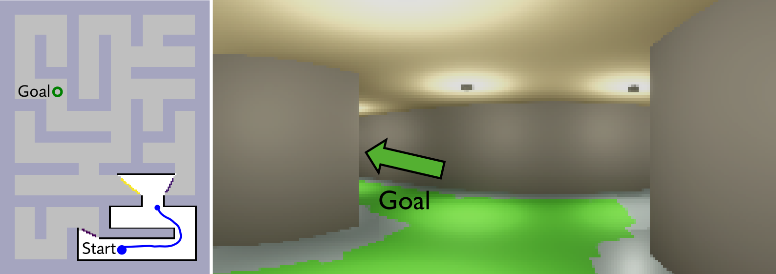
If the robot’s policy in this scenario is to navigate towards the left side of the fork where the floor has a green path, then we know that the robot followed the correct path to the goal. However, if the robot’s policy is to navigate towards the right side of the fork where the floor does not seem to have a green path, we know that the robot will go towards a dead end from which it will have to ultimately backtrack resulting in a greater travel distance.
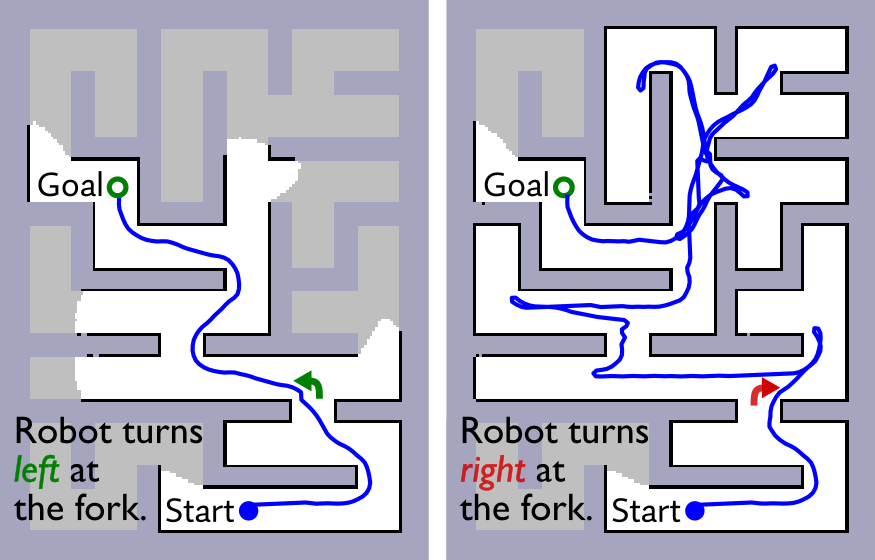
In these two scenarios, we know that any policy that guides the robot towards the right side of the fork will likely result in poor performance compared to a policy that follows the green path at every fork. Indeed, as shown in the figure above, this is what we observe when we deploy the robot with these policies. Given such knowledge, we would want the robot to avoid using a policy that we know will yield a poor performance and select a policy that we know will result in better performance—a problem we refer to as policy selection. The policy that guides the robot towards right goes on to perform even more poorly later on, but the claim still holds even if it had performed better at a later stage during navigation.
The policy that guides the robot towards right goes on to perform even more poorly later on, but the claim still holds even if it had performed better at a later stage during navigation.
However, how can we know which of the policies will result in good performance and which will result in poor performance? Well, we can let the robot deploy each policy one after another and evaluate which of these policies guides the robot to the goal in minimum distance. But, this procedure is costly since we have to deploy the robot multiple times with each policy and wait for it to reach the goal—or fail to do so—before we can determine the best policy, which minimizes distance traveled to reach the goal.
In our work, we develop a procedure that allows a robot to quickly identify which of its policies will result in the best performance upon deployment without having to deploy the robot with all of its policies. Quick identification of the best policy is enabled by our novel offline alt-policy replay approach which effectively allows the robot to imagine what it would have done had it instead used a different policy, thereby sparing the robot from having to deploy all of its policies.
In this article, we discuss our recent IROS 2023 paper Data-Efficient Policy Selection for Navigation in Partial Maps via Subgoal-Based Abstraction which presents a data-efficient policy selection approach in which a robot tasked to navigate to an unseen goal in partially-mapped environments can quickly and reliably identify which of its policies will result in the best performance upon deployment. The article is targeted towards an audience with a basic understanding of robot navigation. However, I will try to provide relevant context or point to resources that might be useful for a more general audience wherever necessary. I have also attached a five-minute video presentation below which covers much of what is discussed in this article. Feel free to check it out before diving into the article.
Policy Selection as an Instance of Multi-armed Bandit Problem
One way of formulating the problem of identifying the best-performing policy from a family of policies is in terms of the multi-armed bandit problem—also known as the model selection problem. A multi-armed bandit problem is a sequential decision-making problem in which an agent must repeatedly choose between a set of actions, each of which has an unknown reward or cost associated with it. The goal of the agent is to maximize the total reward or minimize the total cost it receives over multiple trials. The name multi-armed bandit comes from an old term for slot machines, that each have one arm and steal your money. Multi-armed bandit can be thought of as a set of slot machines: many lever arms each with a different reward scheme.
The name multi-armed bandit comes from an old term for slot machines, that each have one arm and steal your money. Multi-armed bandit can be thought of as a set of slot machines: many lever arms each with a different reward scheme.
Sutton and Barto’s Reinforcement Learning book is a great reference if you want to dive deeper into multi-armed bandit (and RL in general). Here is a link to a PDF of the book the authors make available for free.
Sutton and Barto’s Reinforcement Learning book is a great reference if you want to dive deeper into multi-armed bandit (and RL in general). Here is a link to a PDF of the book the authors make available for free.
One might see that the problem of policy selection is quite similar to the multi-armed bandit problem. In fact, it is an instance of the multi-armed bandit problem. In policy selection, the agent is the robot, the actions are the policies the robot has to select among, and the reward or cost is the performance of the policy measured in terms of the distance traveled by the robot to reach the goal under that policy. The goal of the robot is to minimize the total distance traveled to reach the goal over multiple trials.
Once we instantiate policy selection as a multi-armed bandit problem, we can use bandit algorithms to identify the best-performing policy. For example, consider the well-known Upper Confidence Bound (UCB) bandit algorithm [Lai and Robbins, 1985] to select a policy in trial $k+1$ as described by the equation below.
\[\DeclareMathOperator*{\argmin}{argmin} \pi^{k+1} = \argmin_{\pi \in \mathcal{P}} \Bigg[\bar{C}_k(\pi) - c\sqrt{\cfrac{\ln{k}}{n_k(\pi)}} \,\Bigg]\]Attentive readers may notice that the given equation represents a lower confidence bound (LCB) instead of a UCB since our performance estimates are represented as costs instead of rewards, and is therefore minimized. We use the more common term UCB to mean the approach in general rather than the upper bound itself.
Attentive readers may notice that the given equation represents a lower confidence bound (LCB) instead of a UCB since our performance estimates are represented as costs instead of rewards, and is therefore minimized. We use the more common term UCB to mean the approach in general rather than the upper bound itself.
where, $\mathcal{P}$ is the set of policies to choose from, $\bar{C}_k(\pi)$ is the mean deployment cost of a policy $\pi$ so far, $k$ is the total number of trials completed, $n_k(\pi)$ is the number of times policy $\pi$ has been selected, and $c$ is the exploration parameter.
Intuitively, UCB trades off between selecting the policies with better performance so far, also known as exploitation, and selecting policies that have the potential for better performance, also known as exploration. However, such bandit algorithms are often black-box and generally require the robot to go through multiple deployment trials and incur poor behavior before such policies can be ruled out. This results in very slow convergence towards the best policy and accumulation of large regret. Besides, such a procedure is lengthy and expensive, especially for robot navigation where the result of a navigation trial with a policy is known only after the robot reaches the goal or when it fails to do so.
Accelerating Bandit-like Policy Selection
If we are to accelerate policy selection, we must be able to quickly tighten the bounds on expected performance for each policy, prioritizing the selection of the most promising policies with fewer trials. As such, we seek to constrain policy selection by determining how well an alternative policy could have performed if it had instead been in charge. While we cannot re-deploy the robot to repeat the same trial with another policy, information collected during the trial can be used to scrutinize alternative behaviors and potentially avoid unnecessary exploration. Such a white-box approach can be used to imbue the robot with an ability to introspect the behavior of alternative policies without the need for repeated and costly deployments.
In the section below, we discuss our novel offline alt-policy replay that enables such introspection of the behavior of alternative policies. This allows us to compute a lower bound on the performance of a policy without deploying it in an environment, and thereby more tightly constrain bandit-like selection.
Offline Alt-Policy Replay
In our novel offline alt-policy replay approach, we perform a simulated offline replay of a policy using the information collected by the robot during navigation under a different policy. Specifically, we use the final partial map and the images collected by the robot during a navigation trial to perform simulated navigation of the robot within the boundaries of the partial map with an alternative policy. We say offline replay because the robot doesn’t actually navigate in the environment, it only simulates the navigation based on the information collected during actual navigation.
We say offline replay because the robot doesn’t actually navigate in the environment, it only simulates the navigation based on the information collected during actual navigation.
Such offline replay gives us a lower bound on the deployment cost in case the alternative policy was instead in charge. This means that even after deploying the robot with only one policy, we now have some information about all other policies that can be used to inform bandit-like selection. To accommodate the new lower bound costs of policies computed with offline replay into a bandit-like selection procedure, we propose the Constrained UCB bandit equation as follows.
\[\pi^{k+1} = \argmin_{\pi \in \mathcal{P}} \Bigg[\max \Bigg( C^{\text{lb}}_k(\pi), \bar{C}_k(\pi) - c\sqrt{\cfrac{\ln{k}}{n_k(\pi)}} \,\Bigg)\Bigg]\]where $C^{\text{lb}}_k(\pi)$ is the lower bound on the deployment cost of a policy $\pi$ computed using offline alt-policy replay. Our Constrained UCB bandit policy selection with offline alt-policy replay is illustrated in the figure below.
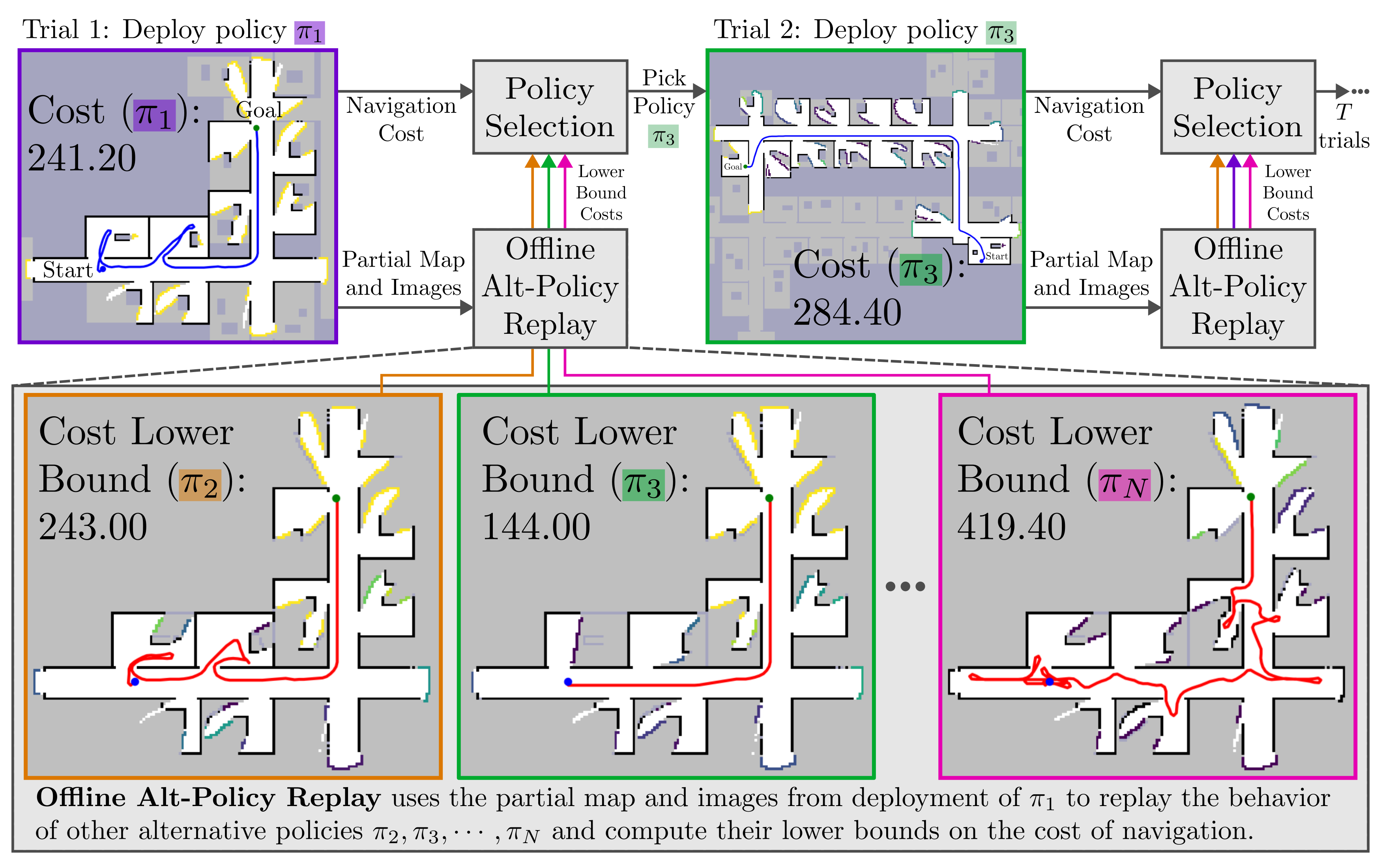
This procedure runs as follows. Before a navigation trial, the robot selects one of the policies and uses it to navigate to the goal.
LSPOffice which was trained in similar office environments and navigates to the goal location with this policy.
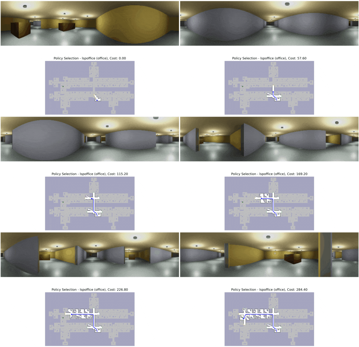
LSPOffice which was trained in similar office environments and navigates to the goal location with this policy.
After the trial is complete, our offline alt-policy replay approach uses the partial map and images collected during the trial to compute lower bounds on the performance of other alternative policies without deploying.
LSPMaze. This policy was trained in maze environments and unsurprisingly performs poorly during offline replay. The lower bound costs are also shown in the figure for reference.
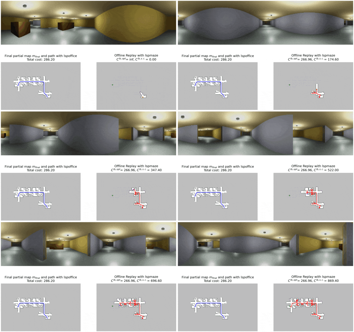
LSPMaze. This policy was trained in maze environments and unsurprisingly performs poorly during offline replay. The lower bound costs are also shown in the figure for reference.
Navigation costs from deployment and lower bound costs from offline alt-policy replay are used by our Constrained UCB bandit policy selection algorithm to pick a policy for the next trial. This process is repeated for multiple trials and the robot keeps picking the most promising policy for every trial.
Not all planning approaches are suitable for offline replay
Scrutinizing alternative behavior to determine the lower bound cost needed for selection via our constrained UCB bandit algorithm requires that we can perform offline alt-policy replay of robot behavior under an alternative policy without actually deploying the robot. In general, replaying a policy offline requires an ability to generate observations from poses the robot may not have visited, which for many learning-informed planning strategies in this domain will not accurately reflect how the policy would have behaved if it had been in control of the robot.
Many approaches to vision-informed navigation under uncertainty, particularly those relying on deep reinforcement learning [Kulhánek et al., 2019, Mirowski et al., 2016], require observations (images) from poses and vantage points not visited during the original trial and can be brittle to even small changes [Henderson et al., 2018], and so replay of such policies is unlikely to yield an accurate lower bound on cost. As such, we instead require an approach to planning that is robust to changes in viewpoint and a kind of policy that is robust to minor changes in robot pose and corresponding observations and can reliably reach the goal even in environments where learning informs poor behavior.
It is our key insight that the Learning over Subgoals Planning (LSP) [Stein et al.] is well-suited for offline alt-policy replay, as it is designed for long-horizon, learning informed planning in partially-mapped environments. In LSP, planning is model-based, and high-level actions correspond to exploration beyond frontiers which represent boundaries between free and unknown space. Learning is used only to make robot-pose-agnostic predictions about the goodness of each such exploratory action: e.g. likelihood that a frontier will lead to the unseen goal.
See our blog post or the LSP paper for more details on the Learning over Subgoals Planning approach.
See our blog post or the LSP paper for more details on the Learning over Subgoals Planning approach.
Since properties of exploratory actions are not dependent on where the robot is, offline replay of LSP-based policies yields accurate lower bounds on their performance making such policies well-suited for offline replay.
Our approach converges faster
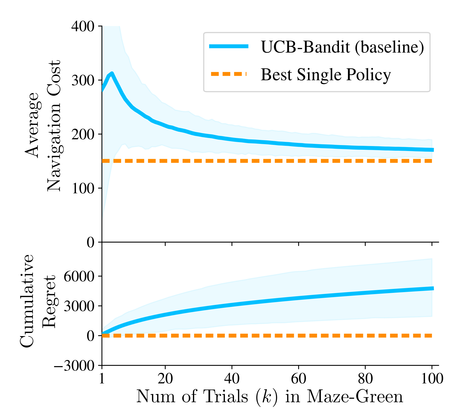
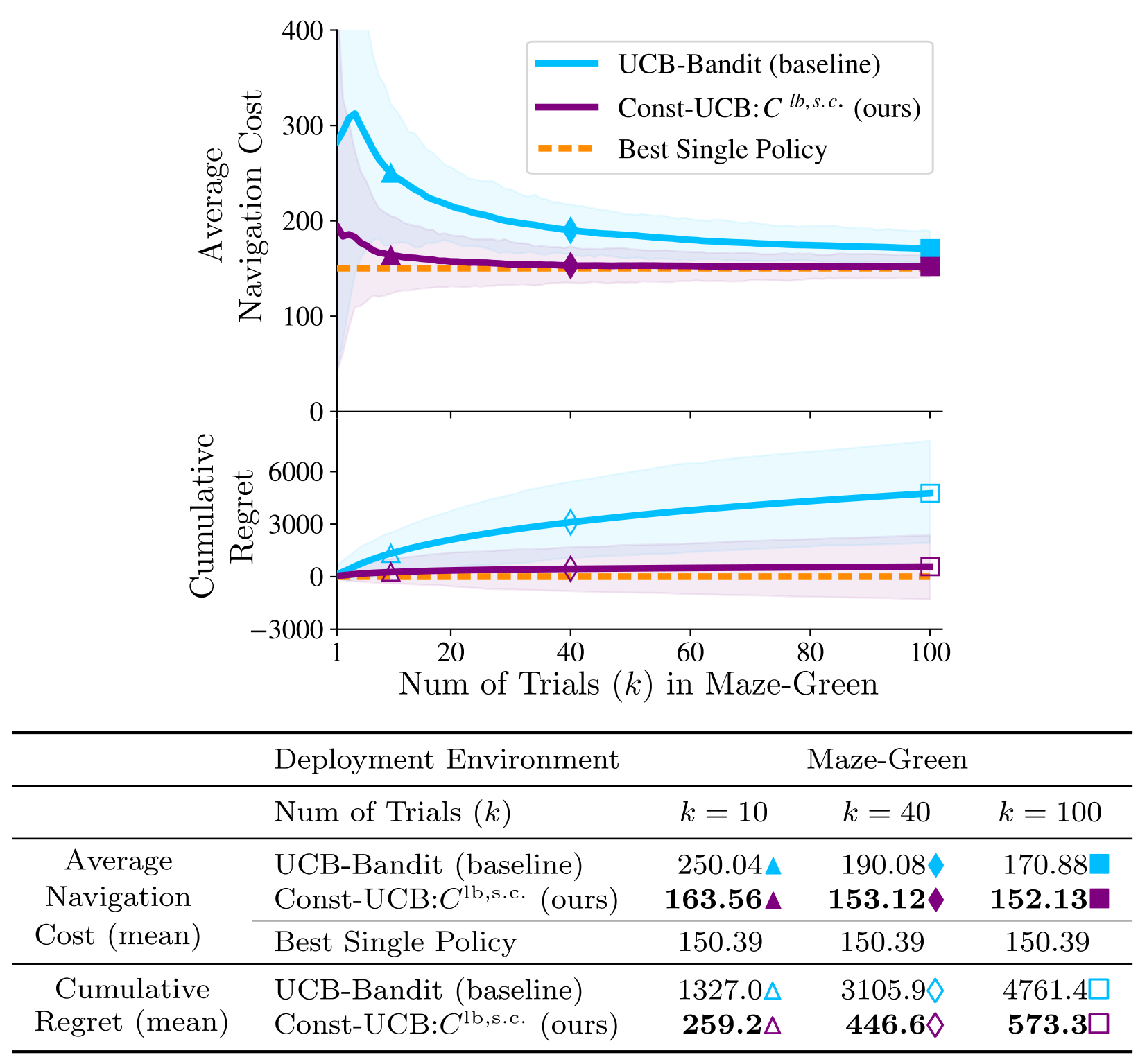
We evaluate our approach in hundreds of simulated maze and office-like environments and compare it with the UCB bandit algorithm. In the figure below, we show results in Maze-Green environments demonstrating that our approach converges much faster than UCB bandit and has 88% lower cumulative regret. See our paper for more results including those in office-like environments.
See our paper for more results including those in office-like environments.
Conclusion and Future Work
We presented a data-efficient policy selection approach that leverages Learning over Subgoals Planning-enabled offline alt-policy replay to compute a lower bound on the performance of policies based on the partial map and images collected from the environment during navigation, and use a bandit-like method to identify the best-performing policy quickly. Our approach enables the learning-guided robot to reduce average navigation cost in a wide variety of partially-mapped environments by picking only those policies that are known to perform better or have the potential to do so thereby significantly reducing the cumulative regret compared to the baseline UCB bandit. In future, we hope to extend our work to perform policy selection with online retraining or adaptation of policies in new environments.
Read our full paper here or feel free to explore our code on GitHub.
Acknowledgements
This material is based upon work supported by the National Science Foundation (NSF) under Grant No. 2232733.

References
- Abhishek Paudel and Gregory J. Stein. Data-Efficient Policy Selection for Navigation in Partial Maps via Subgoal-Based Abstraction. International Conference on Intelligent Robots and Systems (IROS). 2023. paper link
- Lai, Tze Leung, Herbert, Robbins. Asymptotically efficient adaptive allocation rules. Advances in Applied Mathematics. 1985.
- Kulhánek, Jonáš, Erik, Derner, Tim, De Bruin, Robert, Babuška. Vision-based navigation using deep reinforcement learning. European Conference on Mobile Robots (ECMR). 2019.
- Mirowski, Piotr, Razvan, Pascanu, Fabio, Viola, Hubert, Soyer, Andrew J, Ballard, Andrea, Banino, Misha, Denil, Ross, Goroshin, Laurent, Sifre, others. "Learning to navigate in complex environments". arXiv preprint arXiv:1611.03673. 2016.
- Peter Henderson, Riashat Islam, Philip Bachman, Joelle Pineau, Doina Precup, David Meger. Deep Reinforcement Learning that Matters. AAAI Conference on Artificial Intelligence. 2018.
- Stein, Gregory J., Christopher, Bradley, Nicholas, Roy. Learning over Subgoals for Efficient Navigation of Structured, Unknown Environments. Conference on Robot Learning (CoRL). 2018.